import jax, jax.numpy as jnp
from flax import linen as nn
from flax.training import train_state
import optax
import tensorflow_datasets as tfds
import numpy as np
import matplotlib.pyplot as plt
import tensorflow as tf
from tqdm import tqdm
from IPython.display import display, HTML

display(HTML("""
<style>
.output {
    max-height: 300px !important;
    overflow-y: auto !important;
}
div.output_scroll {
    max-height: 300px !important;
}
</style>
"""))
%matplotlib inlineConvolutional Neural Networks
CNN
ML
Deep Learning
Introduction
CNNs are quite common in computer vision tasks. Ranging from simple classification between digits in the MNIST dataset to performing robotic manipulation from vision using Reinforcement Learning. But what are these magical layers that allows us to handle images? What advantages do we get from using them over using standard fully connected layers in MLPs? As we will see in this article CNNs allows us to get better performance with smaller neural network (i.e. less parameters) compared to using fully connected MLPs. Thus making them a suitable candidate for dealing with high dimensional data like images. Convolutions work by passing filters over data extracting features and producing a simpler output.
P.S. this is a stealthy article that also shows you how to write a nice deep learning script for JAX. Googles JIT powered XLA and gradient library.
# The whole data set labels
cifar10_info = tfds.builder('cifar10').info
label_strings = {}
for idx, name in enumerate(cifar10_info.features['label'].names):
    print(f"{idx}: {name}")
    label_strings[idx] = name
0: airplane
1: automobile
2: bird
3: cat
4: deer
5: dog
6: frog
7: horse
8: ship
9: trucknew_label_strings = {}
label_map = {0:0,1:1,2:2,3:3,5:4}
for k, s in label_strings.items():
if label_map.get(k, -1) >= 0: # check if key exists
new_label_strings[label_map[k]] = s
def prepare_dataset(split, batch_size=64, shuffle=True):
    def _filter_and_map(image, label):
        label_map = {0:0, 1:1, 2:2, 3: 3, 5: 4}
        return tf.image.resize(image, [32, 32]) / 255.0, tf.cast(label_map[label.numpy()], tf.int32)

    def _filter(x, y):
        return tf.reduce_any(tf.equal(y, [0, 1, 2, 3, 5]))

    ds = tfds.load('cifar10', split=split, as_supervised=True)
    ds = ds.filter(_filter)
    ds = ds.map(lambda x, y: tf.py_function(_filter_and_map, [x, y], [tf.float32, tf.int32]))
    if shuffle:
        ds = ds.shuffle(1000)
    ds = ds.batch(batch_size).prefetch(1)
    return tfds.as_numpy(ds)
train_ds = prepare_dataset('train')fig, axes = plt.subplots(5, 5, figsize=(6, 6))
axes = axes.flatten()
count = 0
for images, labels in train_ds:
for img, lbl in zip(images, labels):
if count >= 25:
break
ax = axes[count]
ax.imshow(img)
ax.axis('off')
ax.set_title(str(new_label_strings[lbl]), fontsize=8)
count += 1
if count >= 25:
break
# Hide unused subplots
for ax in axes[count:]:
ax.axis('off')
plt.tight_layout()
plt.show()
2025-07-03 23:01:36.290548: W tensorflow/core/kernels/data/cache_dataset_ops.cc:916] The calling iterator did not fully read the dataset being cached. In order to avoid unexpected truncation of the dataset, the partially cached contents of the dataset will be discarded. This can happen if you have an input pipeline similar to `dataset.cache().take(k).repeat()`. You should use `dataset.take(k).cache().repeat()` instead.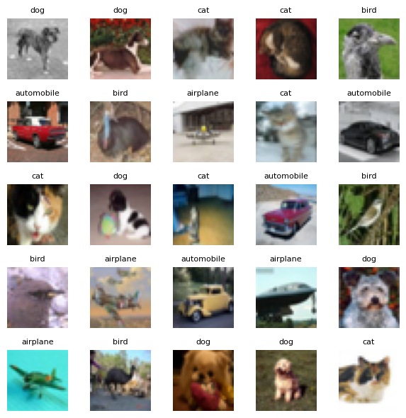
# Get the first batch from train_ds to analyze its dimensions
images, label = next(iter(train_ds))
images.shape, label, label.shape
2025-07-03 23:01:36.825391: W tensorflow/core/kernels/data/cache_dataset_ops.cc:916] The calling iterator did not fully read the dataset being cached. In order to avoid unexpected truncation of the dataset, the partially cached contents of the dataset will be discarded. This can happen if you have an input pipeline similar to `dataset.cache().take(k).repeat()`. You should use `dataset.take(k).cache().repeat()` instead.((64, 32, 32, 3),
array([0, 2, 0, 0, 0, 4, 0, 4, 4, 0, 2, 1, 1, 3, 0, 1, 4, 3, 0, 2, 3, 1,
4, 0, 2, 0, 2, 3, 4, 0, 4, 1, 3, 3, 4, 0, 0, 1, 1, 4, 4, 2, 3, 4,
1, 3, 0, 3, 0, 3, 0, 4, 4, 0, 1, 3, 0, 3, 1, 1, 3, 0, 4, 3],
dtype=int32),
(64,))Defining the MLP
# Let's define out simple MLP with a fully connected hidden layer
class MLP(nn.Module):
    @nn.compact
    def __call__(self, x): # input is a single image of size (width, height, channel)
        x = x.reshape(-1)  # flatten the input image
        x = nn.Dense(256)(x)
        x = nn.relu(x)
        x = nn.Dense(5)(x)
        return x
## This is used to keep track of model params and initialize the model
def create_train_state(rng, model, learning_rate = 1e-3):
params = model.init(rng, jnp.ones([32, 32, 3])) # the second value corrosponds to the model input shape
tx = optax.adam(learning_rate)
return train_state.TrainState.create(apply_fn=model.apply, params=params, tx=tx)## test the MLP on a batch of images
rng = jax.random.PRNGKey(0)
mlp = MLP()
mlp_state = create_train_state(rng, model=mlp)
outputs = jax.vmap(lambda x: mlp_state.apply_fn(mlp_state.params, x))(images)
outputsArray([[ 0.8574835 , 0.2967408 , 0.5020379 , -0.20985158, 0.9080087 ],
[ 0.6394459 , 0.10150381, 0.39180934, -0.14819881, 0.38843006],
[ 0.6392056 , 0.38768694, 0.24764761, -0.50582916, 0.60509944],
[ 0.9406448 , 0.55898184, 0.83870226, -0.2769897 , 0.81999564],
[ 0.5158419 , -0.25098974, 0.30465773, -0.20758504, 0.49279594],
[ 0.6079838 , 0.20021982, 0.65911597, -0.6821174 , 0.26024243],
[ 0.97347176, 0.16529292, 0.49935868, -0.15030667, 1.1000586 ],
[ 0.629176 , 0.3257492 , 0.42310932, -0.06478961, 0.6336051 ],
[ 0.93108976, 0.5870453 , 0.5268865 , -0.23593763, 0.8921703 ],
[ 0.63097376, 0.3136886 , 0.5450499 , -0.22676529, 0.5935381 ],
[ 0.8378334 , 0.24636292, 0.40250263, -0.09808551, 0.7331062 ],
[ 0.81768525, 0.33987695, 0.30860803, -0.19327646, 0.78968006],
[ 0.8786113 , 0.54533434, 0.53306586, -0.46020073, 1.023046 ],
[ 0.93415457, 0.4089566 , 0.31637597, 0.06103394, 1.2814562 ],
[ 1.209869 , 0.4132734 , 0.5195104 , -0.39510572, 1.0848758 ],
[ 0.7246296 , 0.3636866 , 0.24777766, -0.20812212, 0.6078812 ],
[ 0.6755183 , 0.5288818 , 0.36077332, -0.11167393, 0.45888847],
[ 0.2309996 , 0.29093942, 0.17521954, -0.05826601, 0.42536312],
[ 0.6154486 , 0.39786455, 0.7840425 , -0.13525689, 0.6562184 ],
[ 0.65856814, 0.2511847 , 0.3697452 , -0.24171162, 0.4299356 ],
[ 1.2845627 , 0.65384126, 0.48005676, -0.02671895, 1.2014099 ],
[ 1.0398866 , 0.1558535 , 0.44388637, 0.02450314, 0.99380386],
[ 0.8083106 , 0.12910518, 0.42682758, -0.37084585, 0.7035596 ],
[ 0.9273941 , 0.17914855, 0.7214446 , -0.43638453, 1.0167917 ],
[ 1.2740779 , 0.52645767, 0.6796476 , -0.29085398, 1.4282336 ],
[ 0.8479911 , 0.3245369 , 0.85107136, -0.1618606 , 0.6881631 ],
[ 0.44979703, 0.04034848, 0.22773221, -0.05349351, 0.21778208],
[ 0.7978776 , 0.22392118, 0.29038048, -0.15409914, 0.842805 ],
[ 0.61758584, 0.15717185, 0.42102614, -0.2951191 , 0.56094384],
[ 0.9323848 , 0.3481994 , 0.6689151 , -0.43183872, 1.0282344 ],
[ 0.96554255, 0.3094168 , 0.27710545, -0.19069198, 0.7641094 ],
[ 0.9466951 , 0.6974486 , 0.6484781 , -0.00274805, 1.1989698 ],
[ 0.47082758, 0.03498805, 0.49198252, -0.07385243, 0.58799314],
[ 0.97759044, 0.27313852, 0.58677703, -0.46113902, 1.0202582 ],
[ 0.43632135, 0.20464367, 0.37477493, -0.21171832, 0.24368149],
[ 0.7085281 , 0.4206159 , 0.57136494, -0.23627795, 0.88186187],
[ 0.98612946, 0.18416794, 0.40697467, -0.26387995, 0.71193033],
[ 0.77974284, 0.18072803, 0.5959778 , -0.2688065 , 0.67983735],
[ 0.5320593 , -0.03500414, 0.27362183, -0.20494226, 0.2723624 ],
[ 0.7890736 , 0.29375476, 0.4580552 , -0.19813062, 0.7727947 ],
[ 0.72761047, 0.37104407, 0.6217423 , -0.17427173, 0.44040868],
[ 0.926263 , 0.2467773 , 0.5674623 , -0.261243 , 0.600464 ],
[ 0.9612392 , 0.10004815, 0.60566455, -0.34182638, 0.7088696 ],
[ 0.7321015 , 0.28271812, 0.19185676, -0.08365484, 0.54246515],
[ 0.9073818 , 0.34698027, 0.43257883, -0.31254017, 0.5333376 ],
[ 0.6986755 , 0.01641426, 0.5261532 , -0.33697304, 0.531472 ],
[ 0.7314327 , 0.1596696 , 0.55465245, -0.4897889 , 0.79806644],
[ 1.0752794 , -0.04188259, 0.6567116 , -0.38606307, 1.0254107 ],
[ 0.6768588 , 0.28330338, 0.61450386, -0.54482317, 0.8292898 ],
[ 1.0285054 , 0.26882306, 0.5591337 , -0.44829792, 0.8242793 ],
[ 0.5436734 , 0.21320873, 0.5735447 , -0.32222447, 0.6104933 ],
[ 0.51465315, 0.10640214, 0.32332912, -0.34435898, 0.6754335 ],
[ 0.93860745, 0.11113928, 0.5319057 , -0.30059707, 0.7997081 ],
[ 1.1900947 , 0.31101465, 0.7195131 , -0.569692 , 1.1129713 ],
[ 0.4526055 , 0.17554012, 0.3639068 , -0.22404233, 0.42872402],
[ 0.9076593 , 0.15702507, 0.57983756, -0.2339809 , 0.6373191 ],
[ 0.65093136, 0.2736031 , 0.36151338, -0.226747 , 0.27226087],
[ 0.7891079 , 0.4474245 , 0.5419042 , -0.11550926, 0.67835516],
[ 0.554339 , 0.47481042, 0.1299768 , -0.12698087, 0.6532611 ],
[ 0.87211895, 0.43963614, 0.39935672, -0.18192181, 0.6740452 ],
[ 1.068575 , 0.15600765, 0.697804 , -0.48420894, 0.9931273 ],
[ 0.8187059 , 0.34735546, 0.6780616 , -0.36486238, 0.93379873],
[ 0.6570326 , 0.19099687, 0.46740726, -0.4876986 , 0.5763815 ],
[ 0.98657477, 0.28399062, 0.80063576, -0.41992465, 0.85719055]], dtype=float32)## ALWAYS MAKE SURE OUTPUT DIMENSIONS MAKE SENSE!
assert outputs.shape == (64,5)class CNN(nn.Module):
@nn.compact
def __call__(self, x):
x = nn.Conv(32, (3,3))(x)
x = nn.relu(x)
x = nn.avg_pool(x, (2,2), (2,2))
x = nn.Conv(64, (3,3))(x)
x = nn.relu(x)
x = nn.avg_pool(x, (2,2), (2,2))
# MLP architecture from here on-wards
x = x.reshape(-1)
x = nn.Dense(128)(x)
x = nn.relu(x)
x = nn.Dense(5)(x)
return xrng = jax.random.PRNGKey(0)
cnn = CNN()
cnn_state = create_train_state(rng, model=cnn)
output = jax.vmap(lambda x: cnn_state.apply_fn(cnn_state.params, x))(images) # default axis is batch dimension (axis = 0)
outputArray([[ 4.33102585e-02, -2.24208698e-01, 1.22603446e-01,
-1.50668398e-01, 2.05121949e-01],
[ 5.57019608e-03, -8.16603377e-03, 9.35379267e-02,
-1.08800054e-01, 1.20641910e-01],
[ 9.50803012e-02, -1.26184836e-01, 1.72937065e-01,
-4.08819430e-02, 1.93043739e-01],
[ 1.03128754e-01, -5.72365783e-02, 2.50474840e-01,
-9.90523174e-02, 2.09798515e-01],
[ 1.31292775e-01, 6.67526200e-03, 1.49251387e-01,
-7.65084550e-02, 2.07161099e-01],
[ 2.43950114e-02, 8.60773325e-02, 1.22257218e-01,
-1.17454275e-01, 2.22982705e-01],
[ 4.13091481e-03, -1.33933306e-01, 1.85999215e-01,
-1.16527379e-01, 2.44172111e-01],
[ 2.95359045e-02, -6.55516833e-02, 1.17702857e-01,
-2.53058262e-02, 1.76266387e-01],
[ 6.78401515e-02, -7.50230774e-02, 2.32504979e-01,
-5.43524325e-02, 3.07944685e-01],
[ 3.95299867e-02, 4.17144783e-03, 1.33808404e-01,
-3.27123031e-02, 2.52673358e-01],
[ 1.30284065e-02, -6.05607592e-02, 1.28177673e-01,
-9.12525654e-02, 1.99974552e-01],
[ 4.37443070e-02, -5.38351387e-02, 9.29535404e-02,
-1.34287685e-01, 2.06874683e-01],
[ 9.85109508e-02, -1.66002110e-01, 1.50731415e-01,
-2.05984905e-01, 2.56021082e-01],
[ 2.46936101e-02, -4.82751355e-02, 1.95547462e-01,
-5.77657409e-02, 2.56542504e-01],
[ 7.76570365e-02, -1.39449745e-01, 2.69246072e-01,
-1.08291052e-01, 3.17445844e-01],
[ 1.00872353e-01, -7.57703632e-02, 9.91501361e-02,
-7.18758851e-02, 1.32879242e-01],
[-2.69391853e-02, 2.18723360e-02, 1.16466410e-01,
-6.62022084e-02, 1.65445894e-01],
[ 5.66744246e-02, -9.24601331e-02, 1.02567926e-01,
-1.00574128e-01, 1.45497888e-01],
[ 1.61505118e-01, 8.01496021e-03, 1.90237775e-01,
-6.58064485e-02, 2.45871812e-01],
[ 4.87874709e-02, -3.36904894e-04, 1.59409046e-01,
-7.41260722e-02, 1.56417429e-01],
[ 6.91207051e-02, -8.44717249e-02, 1.17989093e-01,
-4.05639000e-02, 2.51733512e-01],
[ 6.85547572e-03, -3.28061506e-02, 2.00641721e-01,
-1.88892186e-01, 1.78098962e-01],
[ 1.96740890e-04, -1.23728536e-01, 1.48138911e-01,
-1.10798106e-01, 1.32907733e-01],
[ 9.57120061e-02, -3.34039107e-02, 1.31730169e-01,
-9.14398208e-02, 2.40440562e-01],
[ 8.08523968e-02, -7.17288777e-02, 2.39552438e-01,
-1.37980193e-01, 3.68334442e-01],
[ 6.93092570e-02, -3.00794132e-02, 1.48313105e-01,
-2.68042963e-02, 2.04498827e-01],
[ 4.93414216e-02, -1.26811424e-02, 1.45047024e-01,
-1.36372978e-02, 1.29502803e-01],
[-4.96724173e-02, -3.49755473e-02, 1.03962861e-01,
-1.24199122e-01, 2.48753935e-01],
[ 3.31715159e-02, 4.09440463e-03, 1.68211326e-01,
-4.06639688e-02, 2.17514843e-01],
[ 1.11712448e-01, -7.14526772e-02, 2.09489182e-01,
-7.87913352e-02, 3.05470139e-01],
[ 4.62175049e-02, -8.09207857e-02, 1.33963987e-01,
-1.13125898e-01, 1.70414999e-01],
[ 5.78913875e-02, -1.43240476e-02, 1.36690766e-01,
-1.28760710e-01, 2.86878705e-01],
[ 6.54461607e-02, 2.51243971e-02, 2.04747900e-01,
-8.11515898e-02, 2.04848215e-01],
[ 4.16154377e-02, -1.00531116e-01, 1.84638023e-01,
-1.26019031e-01, 3.10940534e-01],
[ 9.44609195e-02, -4.02740091e-02, 1.60891727e-01,
-2.10279264e-02, 1.82557508e-01],
[ 7.22014010e-02, -1.24151789e-01, 1.72335356e-01,
-1.29979014e-01, 2.64235556e-01],
[ 3.65216099e-02, 1.66072380e-02, 1.43591866e-01,
-6.17942028e-02, 1.77656561e-01],
[ 7.35495836e-02, -9.21484083e-02, 1.50036827e-01,
-1.39586210e-01, 2.11914703e-01],
[ 2.08473355e-02, 9.38035026e-02, 9.11838412e-02,
-4.82535474e-02, 1.44369915e-01],
[ 4.45854068e-02, -6.75124079e-02, 1.26784205e-01,
-1.19716667e-01, 1.75546721e-01],
[ 3.80449109e-02, 1.80718135e-02, 1.91719040e-01,
-4.64373901e-02, 3.04098994e-01],
[ 4.54951152e-02, -8.15637857e-02, 1.55733287e-01,
-1.16467893e-01, 2.41689011e-01],
[ 3.45387049e-02, -2.04511974e-02, 1.93799406e-01,
-1.43637910e-01, 2.63246000e-01],
[-1.02505125e-01, -5.42742014e-02, 8.49395171e-02,
-9.21501592e-02, 1.03385307e-01],
[-1.24675152e-03, -1.28563112e-02, 9.78402570e-02,
-1.35453671e-01, 1.62125885e-01],
[ 2.85631679e-02, 2.66707921e-03, 1.86013639e-01,
-5.22268564e-02, 2.35220268e-01],
[ 1.45691186e-01, -3.40135209e-02, 2.17030197e-01,
-6.22520670e-02, 2.34056249e-01],
[ 3.56792249e-02, 2.26562936e-02, 2.68988878e-01,
-4.48365510e-02, 3.61441731e-01],
[ 1.64968506e-01, 1.78313069e-03, 2.39997447e-01,
-2.31388900e-02, 2.93607473e-01],
[-6.06130026e-02, -6.29288480e-02, 1.65078804e-01,
-1.65459543e-01, 2.87701428e-01],
[ 1.39888212e-01, -1.93722325e-03, 1.96833193e-01,
1.55947311e-03, 2.09751830e-01],
[ 2.75153313e-02, -6.83044717e-02, 2.02807695e-01,
-7.20612332e-02, 2.38654122e-01],
[ 2.56417207e-02, 5.39707653e-02, 1.22497432e-01,
-1.45303570e-02, 2.55295873e-01],
[ 4.36963104e-02, -3.62206101e-02, 2.62431800e-01,
-4.47982959e-02, 3.00564528e-01],
[ 6.39088377e-02, -1.23333395e-01, 7.03526214e-02,
-6.83718771e-02, 1.22903541e-01],
[-3.89707908e-02, -4.74605002e-02, 1.43152639e-01,
-5.27028888e-02, 2.72179127e-01],
[ 8.09255317e-02, -5.85454553e-02, 1.14749864e-01,
-3.25130895e-02, 2.46704489e-01],
[ 5.61878048e-02, -6.82451054e-02, 1.64389834e-01,
-4.19153981e-02, 1.98826119e-01],
[-2.79332846e-02, -3.00862342e-02, 1.06392294e-01,
-5.01194224e-02, 7.07748383e-02],
[ 7.81371370e-02, -9.86558422e-02, 1.48843333e-01,
-2.11230721e-02, 1.61438674e-01],
[ 5.27138487e-02, -8.32521468e-02, 2.69904405e-01,
-1.00137964e-01, 3.85229498e-01],
[ 1.60061255e-01, 3.36131789e-02, 2.27109954e-01,
-2.54349448e-02, 3.27930987e-01],
[ 6.07025549e-02, -5.71473688e-02, 1.27371192e-01,
-7.98806548e-02, 1.45142466e-01],
[ 1.04193404e-01, -9.55243781e-02, 3.35441500e-01,
-4.20354344e-02, 4.02535856e-01]], dtype=float32)assert outputs.shape == (64, 5)Define the loss function
This is the measure of performance for our artifical neural network. It needs to be designed in a way that is sound and can be optimized using convex optimization and gradient descent. For the purposes of classification we can use cross-entropy loss:
The cross-entropy loss can be interpreted as the sum of the entropy of the true distribution and the Kullback-Leibler (KL) divergence between the true distribution \(y\) and the predicted distribution \(\hat{y}\):
\[ \mathcal{L}_{\text{CE}}(y, \hat{y}) = H(y) + D_{\mathrm{KL}}(y \parallel \hat{y}) \]
where
\[ D_{\mathrm{KL}}(y \parallel \hat{y}) = \sum_{i=1}^C y_i \log\left(\frac{y_i}{\hat{y}_i}\right) \]
and \(H(y)\) is the entropy of the true distribution. In classification, \(H(y)\) is constant, so minimizing cross-entropy is equivalent to minimizing the KL divergence.
The cross-entropy loss for a classification problem with \(C\) classes is defined as:
\[ \mathcal{L}_{\text{CE}} = -\sum_{i=1}^C y_i \log(\hat{y}_i) \]
where \(y_i\) is the true label (one-hot encoded) and \(\hat{y}_i\) is the predicted probability for class \(i\).
For a batch of \(N\) samples, the average cross-entropy loss is:
\[ \mathcal{L}_{\text{batch}} = -\frac{1}{N} \sum_{n=1}^N \sum_{i=1}^C y_{n,i} \log(\hat{y}_{n,i}) \]
# let's test the loss function to check it out
l = optax.softmax_cross_entropy_with_integer_labels(logits=outputs, labels=labels).mean()
lArray(1.702628, dtype=float32)Put it all together
## define the network architectures
## MLP ##
class MLP(nn.Module):
@nn.compact
def __call__(self, x): # input is a single image of size (width, height, channel)
x = x.reshape(-1) # flatten the input image
x = nn.Dense(256)(x)
x = nn.relu(x)
x = nn.Dense(256)(x)
x = nn.relu(x)
x = nn.Dense(5)(x)
return x
## CNN ##
class CNN(nn.Module):
    @nn.compact
    def __call__(self, x):
        x = nn.Conv(32, (3,3))(x)
        x = nn.relu(x)
        x = nn.avg_pool(x, (2,2), (2,2))
        x = nn.Conv(64, (3,3))(x)
        x = nn.relu(x)
        x = nn.avg_pool(x, (2,2), (2,2))
        # MLP architecture from here on-wards
        x = x.reshape(-1)
        x = nn.Dense(128)(x)
        x = nn.relu(x)
        x = nn.Dense(5)(x)
        return x
def create_train_state(rng, model, learning_rate = 1e-3):
    params = model.init(rng, jnp.ones([32, 32, 3])) # the second value corrosponds to the model input shape
    tx = optax.adam(learning_rate)
    return train_state.TrainState.create(apply_fn=model.apply, params=params, tx=tx)
def compute_eval_metrics(logits, labels):
loss = optax.softmax_cross_entropy_with_integer_labels(logits, labels).mean()
accuracy = jnp.mean(jnp.argmax(logits, -1) == labels)
return loss, accuracy
@jax.jit
def train_step(state, batch):
    images, labels = batch
    def loss_fn(params):
        logits = jax.vmap(lambda x: state.apply_fn(params, x))(images)
        loss = optax.softmax_cross_entropy_with_integer_labels(logits, labels).mean()
        return loss, logits

    grad_fn = jax.value_and_grad(loss_fn, has_aux=True)
    (loss, logits), grads = grad_fn(state.params)
    state = state.apply_gradients(grads=grads)
    acc = jnp.mean(jnp.argmax(logits, -1) == labels)
    return state, loss, acc
rng = jax.random.PRNGKey(0)
batch_data = next(iter(train_ds))
cnn = CNN()
cnn_state = create_train_state(rng, cnn)
_ = train_step(state=cnn_state, batch=batch_data)2025-07-03 23:10:31.612581: W tensorflow/core/kernels/data/cache_dataset_ops.cc:916] The calling iterator did not fully read the dataset being cached. In order to avoid unexpected truncation of the dataset, the partially cached contents of the dataset will be discarded. This can happen if you have an input pipeline similar to `dataset.cache().take(k).repeat()`. You should use `dataset.take(k).cache().repeat()` instead.
def eval_step(params, batch, apply_fn):
    imgs, labels = batch
    logits = jax.vmap(lambda x: apply_fn(params, x))(imgs)
    return compute_eval_metrics(logits, labels)
def train(model, train_ds, epochs = 50, seed=0):
rng = jax.random.PRNGKey(seed)
state = create_train_state(rng, model)
train_losses = []
train_accuracies = []
pbar = tqdm(range(epochs), desc="Epochs") # progress bar
for epoch in pbar:
epoch_loss, epoch_acc, count = 0, 0, 0
for batch in train_ds:
state, loss, accuracy = train_step(state, batch)
batch_size = len(batch[1])
epoch_loss += loss * batch_size
epoch_acc += accuracy * batch_size
count += batch_size
train_losses.append(epoch_loss / count)
train_accuracies.append(epoch_acc / count)
pbar.set_postfix({
"train_loss": float(train_losses[-1]),
"train_acc": float(train_accuracies[-1])
})
return state, train_losses, train_accuracies
def eval(state, test_ds):
    test_loss, test_accuracy, count = 0, 0, 0

    for batch in test_ds:

        loss, acc = eval_step(state.params, batch, state.apply_fn)
        batch_size = len(batch[1])
        test_loss += loss * batch_size
        test_accuracy += acc * batch_size
        count += batch_size
    test_loss /= count
    test_accuracy /= count
    return test_accuracy, test_loss
train_ds = prepare_dataset('train')
test_ds = prepare_dataset('test', shuffle=False)## Train MLP Classifier
mlp = MLP()
mlp_state, mlp_train_losses, mlp_train_accuracies = train(model=mlp, train_ds=train_ds, epochs=30)Epochs: 100%|██████████| 30/30 [03:35<00:00, 7.19s/it, train_loss=0.708, train_acc=0.714]## Train MLP Classifier
cnn = CNN()
cnn_state, cnn_train_losses, cnn_train_accuracies = train(model=cnn, train_ds=train_ds, epochs=30)Epochs: 100%|██████████| 30/30 [05:19<00:00, 10.65s/it, train_loss=0.0461, train_acc=0.985]Results
# Plot Everything
epochs = range(1, len(mlp_train_losses)+1)
plt.figure(figsize=(12,5))
plt.subplot(1,2,1)
plt.plot(epochs, mlp_train_accuracies, label='MLP')
plt.plot(epochs, cnn_train_accuracies, label='CNN')
plt.ylabel("Accuracy"); plt.xlabel("Epoch"); plt.title("Training Accuracy")
plt.legend()

plt.subplot(1,2,2)
plt.plot(epochs, mlp_train_losses, label='MLP')
plt.plot(epochs, cnn_train_losses, label='CNN')
plt.ylabel("Loss"); plt.xlabel("Epoch"); plt.title("Training Loss")
plt.legend()
plt.tight_layout()
plt.show()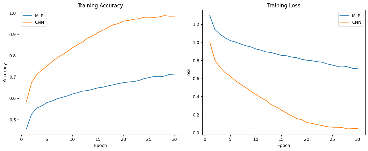
test_accuracy, test_loss = eval(mlp_state, test_ds)
print(f"MLP Test Accuracy: {test_accuracy:.4f}")
print(f"MLP Test Loss: {test_loss:.4f}")
MLP Test Accuracy: 0.5934
MLP Test Loss: 1.0474cnn_test_accuracy, cnn_test_loss = eval(cnn_state, test_ds)
print(f"CNN Test Accuracy: {cnn_test_accuracy:.4f}")
print(f"CNN Test Loss: {cnn_test_loss:.4f}")MLP Test Accuracy: 0.7492
MLP Test Loss: 1.5188print(mlp.tabulate(rng, jnp.ones([32,32,3])))MLP Summary ┏━━━━━━━━━┳━━━━━━━━┳━━━━━━━━━━━━━━━━━━┳━━━━━━━━━━━━━━┳━━━━━━━━━━━━━━━━━━━━━━━━━┓ ┃ path ┃ module ┃ inputs ┃ outputs ┃ params ┃ ┡━━━━━━━━━╇━━━━━━━━╇━━━━━━━━━━━━━━━━━━╇━━━━━━━━━━━━━━╇━━━━━━━━━━━━━━━━━━━━━━━━━┩ │ │ MLP │ float32[32,32,3] │ float32[5] │ │ ├─────────┼────────┼──────────────────┼──────────────┼─────────────────────────┤ │ Dense_0 │ Dense │ float32[3072] │ float32[256] │ bias: float32[256] │ │ │ │ │ │ kernel: │ │ │ │ │ │ float32[3072,256] │ │ │ │ │ │ │ │ │ │ │ │ 786,688 (3.1 MB) │ ├─────────┼────────┼──────────────────┼──────────────┼─────────────────────────┤ │ Dense_1 │ Dense │ float32[256] │ float32[256] │ bias: float32[256] │ │ │ │ │ │ kernel: │ │ │ │ │ │ float32[256,256] │ │ │ │ │ │ │ │ │ │ │ │ 65,792 (263.2 KB) │ ├─────────┼────────┼──────────────────┼──────────────┼─────────────────────────┤ │ Dense_2 │ Dense │ float32[256] │ float32[5] │ bias: float32[5] │ │ │ │ │ │ kernel: float32[256,5] │ │ │ │ │ │ │ │ │ │ │ │ 1,285 (5.1 KB) │ ├─────────┼────────┼──────────────────┼──────────────┼─────────────────────────┤ │ │ │ │ Total │ 853,765 (3.4 MB) │ └─────────┴────────┴──────────────────┴──────────────┴─────────────────────────┘ Total Parameters: 853,765 (3.4 MB)
print(cnn.tabulate(rng, jnp.ones([32,32,3])))CNN Summary ┏━━━━━━━━━┳━━━━━━━━┳━━━━━━━━━━━━━━━━━━━┳━━━━━━━━━━━━━━━━━━━┳━━━━━━━━━━━━━━━━━━━┓ ┃ path ┃ module ┃ inputs ┃ outputs ┃ params ┃ ┡━━━━━━━━━╇━━━━━━━━╇━━━━━━━━━━━━━━━━━━━╇━━━━━━━━━━━━━━━━━━━╇━━━━━━━━━━━━━━━━━━━┩ │ │ CNN │ float32[32,32,3] │ float32[5] │ │ ├─────────┼────────┼───────────────────┼───────────────────┼───────────────────┤ │ Conv_0 │ Conv │ float32[32,32,3] │ float32[32,32,32] │ bias: float32[32] │ │ │ │ │ │ kernel: │ │ │ │ │ │ float32[3,3,3,32] │ │ │ │ │ │ │ │ │ │ │ │ 896 (3.6 KB) │ ├─────────┼────────┼───────────────────┼───────────────────┼───────────────────┤ │ Conv_1 │ Conv │ float32[16,16,32] │ float32[16,16,64] │ bias: float32[64] │ │ │ │ │ │ kernel: │ │ │ │ │ │ float32[3,3,32,6… │ │ │ │ │ │ │ │ │ │ │ │ 18,496 (74.0 KB) │ ├─────────┼────────┼───────────────────┼───────────────────┼───────────────────┤ │ Dense_0 │ Dense │ float32[4096] │ float32[128] │ bias: │ │ │ │ │ │ float32[128] │ │ │ │ │ │ kernel: │ │ │ │ │ │ float32[4096,128] │ │ │ │ │ │ │ │ │ │ │ │ 524,416 (2.1 MB) │ ├─────────┼────────┼───────────────────┼───────────────────┼───────────────────┤ │ Dense_1 │ Dense │ float32[128] │ float32[5] │ bias: float32[5] │ │ │ │ │ │ kernel: │ │ │ │ │ │ float32[128,5] │ │ │ │ │ │ │ │ │ │ │ │ 645 (2.6 KB) │ ├─────────┼────────┼───────────────────┼───────────────────┼───────────────────┤ │ │ │ │ Total │ 544,453 (2.2 MB) │ └─────────┴────────┴───────────────────┴───────────────────┴───────────────────┘ Total Parameters: 544,453 (2.2 MB)
Two things standout: - CNN outperforms MLP in classification - CNN is able to do this with less number of parameters
Save model parameters for future work
from flax.serialization import to_bytes

# Save MLP model parameters
with open("mlp_params.msgpack", "wb") as f:
    f.write(to_bytes(mlp_state.params))

# Save CNN model parameters
with open("cnn_params.msgpack", "wb") as f:
    f.write(to_bytes(cnn_state.params))
Load model and test on an image from the internet
from flax.serialization import from_bytes
with open("cnn_params.msgpack", "rb") as f:
    cnn_params = from_bytes(cnn_state.params, f.read())
from PIL import Image
# load and view the image
# Replace 'your_image.jpg' with your image file path
img = Image.open('../images/cat.jpg')
plt.imshow(img)
plt.axis('off')
plt.show()
## Process Image so that it fits our neural net architecture
img_resized = img.resize((32, 32))
plt.imshow(img_resized)
plt.axis('off')
plt.show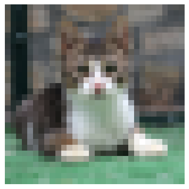
## Now run inference on the image to predict its label

prediction = cnn_state.apply_fn(cnn_params, jnp.array(img_resized))
prediction, nn.softmax(prediction)
(Array([ -777.1376, -2318.708 , -6668.267 , 2252.1262, 1919.2493], dtype=float32),
Array([0., 0., 0., 1., 0.], dtype=float32))label_index = jnp.argmax(nn.softmax(prediction))
new_label_strings[int(label_index)]'cat'## Let's predict the label for two images and display them side by side
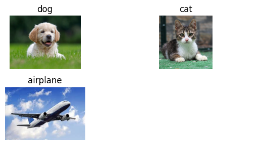
test_images = {
"dog_img" : Image.open("../images/dog.jpg"),
"cat_img" : Image.open("../images/cat.jpg"),
"plane_img" : Image.open("../images/plane.jpg")
}
fig, axes = plt.subplots(2, 2, figsize=(6, 3))
## Dog image ##
dog_img_resized = test_images["dog_img"].resize((32, 32))
inference = nn.softmax(cnn_state.apply_fn(cnn_params, jnp.array(dog_img_resized)))
prediction = int(jnp.argmax(inference))
axes[0][0].imshow(test_images["dog_img"])
axes[0][0].set_title(new_label_strings[prediction])
axes[0][0].axis('off')
## Cat image ##
dog_img_resized = test_images["cat_img"].resize((32, 32))
inference = nn.softmax(cnn_state.apply_fn(cnn_params, jnp.array(dog_img_resized)))
prediction = int(jnp.argmax(inference))
axes[0][1].imshow(test_images["cat_img"])
axes[0][1].set_title(new_label_strings[prediction])
axes[0][1].axis('off')
## Plane image ##
dog_img_resized = test_images["plane_img"].resize((32, 32))
inference = nn.softmax(cnn_state.apply_fn(cnn_params, jnp.array(dog_img_resized)))
prediction = int(jnp.argmax(inference))
axes[1][0].imshow(test_images["plane_img"])
axes[1][0].set_title(new_label_strings[prediction])
axes[1][0].axis('off')
axes[1][1].axis('off')
plt.tight_layout()
plt.show()