Inverse Kinematics: Pose from Point instead of Point from Pose

Introduction

Point at your nose. In how many ways can you orient your arm and index finger to accomplish this?

Why am I asking you this? As humans, we move our arms naturally and effortlessly to perform such tasks, but robotic arms do not have this intuitive ability. For a robot, specifying a hand (an end-effector) position requires providing the exact joint angles and orientation. This would be tedious if humans had to consciously think about the precise angles of our elbows or shoulders every time we moved. In robotics, one common method for achieving a desired end-effector position is called inverse kinematics.

In inverse kinematics, we are given a desired end-effector position and must determine the joint angles that achieve it—if such a configuration exists. For example, as in the nose-pointing scenario, there are many possible ways to arrange your arm to reach the same point. On the contrary, if you are asked to place your hand on the ceiling without assistance, it may be physically impossible. In mathematical terms, this means that an exact solution to the inverse kinematics problem may not exist if the target position is outside the robot’s reachable workspace.

General Formulation of Inverse Kinematics

A forward kinematics function maps from joint angles (\(\mathbf{q} \in \mathbb{R}^n\)) to gripper position (\(\mathbf{x} \in \mathbb{R}^3\)):

\[ \mathbf{x} = f(\mathbf{q}) \]

In inverse kinematics, we want to find \(\mathbf{q}^*\) such that it satisfies the following optimization problem:

\[ \mathbf{q}^* = \underset{\mathbf{q}}{\operatorname{argmin}}\, \lVert f(\mathbf{q}) - \mathbf{x}_{\text{target}} \rVert \]

The Jacobian of a robotic manipulator relates joint velocities (\(\dot{\mathbf{q}}\)) to end-effector velocities (\(\dot{\mathbf{x}}\)):

\[ \dot{\mathbf{x}} = \mathbf{J}(\mathbf{q})\, \dot{\mathbf{q}} \]

We can use the pseudo-inverse of the Jacobian to perform inverse kinematics:

\[ \dot{\mathbf{q}} = \mathbf{J}(\mathbf{q})^\dagger\, \dot{\mathbf{x}} \]

And then solve this equation using numerical and iterative methods.

\begin{algorithm} \caption{Iterative Inverse Kinematics Using Jacobian Pseudoinverse} \begin{algorithmic} \State Start with initial joint angles $\theta$ \Repeat \State Compute end-effector position $x = f(\theta)$ \State Compute error $\delta = x_{target} - x$ \State Compute Jacobian $J(\theta)$ \State Compute update $\Delta\theta = J^{\dagger} \delta$ \State Update angles $\theta \gets \theta + \alpha \Delta\theta$ \Until{$||\delta||$ < $\epsilon$} \end{algorithmic} \end{algorithm}

Example: 2D and 2 links

Here’s a sample implementation of performing inverse kinematics using an iterative least-squares method described above:

import numpy as np
import matplotlib.pyplot as plt

def plot_trajectories(trajectory):
  assert np.linalg.norm(delta) <= 0.01 
  plt.figure(figsize=(6, 6))
  for index, arm in enumerate(trajectory):
    if index % 500 == 0:
      # Plot both links for each sampled pose
      plt.plot([0, arm[0,0]], [0, arm[1,0]], '--', color='gray', alpha=0.3)  # Link 1
      plt.plot([arm[0,0], arm[0,1]], [arm[1,0], arm[1,1]], '--', color='gray', alpha=0.3)  # Link 2
  # Final pose
  final = trajectory[-1]
  plt.plot([0, final[0,0]], [0, final[1,0]], 'o-', color='blue', linewidth=2, label='Link 1 (final)')
  plt.plot([final[0,0], final[0,1]], [final[1,0], final[1,1]], 'o-', color='green', linewidth=2, label='Link 2 (final)')
  plt.plot(target[0], target[1], 'rx', markersize=10, label='Target')
  plt.xlim(0.0, 1.5)
  plt.ylim(0.0, 1.5)
  plt.gca().set_aspect('equal')
  plt.grid(True)
  plt.legend()
  plt.title("IK trajectories")
  plt.show()

def forward_kinematics(theta1, theta2, l1=1.0, l2=1.0):
    x1 = l1 * np.cos(theta1)
    y1 = l1 * np.sin(theta1)
    x2 = x1 + l2 * np.cos(theta1 + theta2)
    y2 = y1 + l2 * np.sin(theta1 + theta2)
    return np.array([[x1, x2], [y1, y2]])

def jacobian(theta1, theta2, l1=1.0, l2=1.0):
    j11 = -l1*np.sin(theta1) - l2*np.sin(theta1 + theta2)
    j12 = -l2*np.sin(theta1 + theta2)
    j21 =  l1*np.cos(theta1) + l2*np.cos(theta1 + theta2)
    j22 =  l2*np.cos(theta1 + theta2)
    return np.array([[j11, j12], [j21, j22]])

## IK ##

theta = np.array([0.5, 0.5])
trajectory = []
delta = np.inf
epsilon = 0.01 # success threshold
target = np.array([1.2, 1.3])
# link lengths set to 1m
l1 = 1.0
l2 = 1.0 

alpha = 0.001
while np.linalg.norm(delta) > epsilon:
  link_pos_estimates = forward_kinematics(theta[0], theta[1], l1, l2)
  trajectory.append(link_pos_estimates.copy())
  ee_pos_estimate = link_pos_estimates[:,-1]
  delta = target - ee_pos_estimate
  Jac = jacobian(theta[0], theta[1],l1 ,l2)

  delta_theta = np.linalg.pinv(Jac).dot(delta)

  theta += alpha*delta_theta

plot_trajectories(trajectory)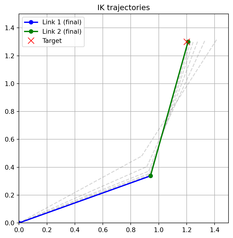

Future work

In this post, I only covered the base case of inverse kinematics. This can be extended to additional links and 3D space. Stay tuned for more content!